The PPMT Function is categorized under Excel Financial functions. The function will calculate the payment on the principal for a loan or an investment based on periodic, constant payments and a fixed interest rate for a given period of time.
In financial analysis, the PPMT function is useful in understanding the primary components of the total payments made for a loan taken.
Formula
=PPMT( rate, per, nper, pv, [fv], [type] )
The PPMT function uses the following arguments:
- Rate (required argument) – This is the interest rate per period.
- Per (required argument) – A bond’s maturity date, that is, the date when bond expires.
- Nper (required argument) – The total number of payment periods.
- Pv (required argument) – This is the present value of the loan/investment. It is the total amount that a series of future payments is worth now.
- Fv (optional argument) – Specifies the future value of the loan/investment at the end of nper payments. If omitted, [fv] takes on the default value of 0.
- Type (optional argument) – This specifies whether the payment is made at the start or the end of the period. It can assume a value of 0 or 1. If it is 0, it means the payment is made at the end of the period, and if 1, the payment is made at the start. If we omit the [type] argument, it will take on the default value of 0, denoting payments made at the end of the period.
How to use the PPMT Function in Excel?
As a worksheet function, PPMT can be entered as part of a formula in a cell of a worksheet. To understand the uses of the function, let us consider an example:
<amp-ad width="100vw" height="320"
type="adsense"
data-ad-client="ca-pub-8221744489009306"
data-ad-slot="8195628836"
data-auto-format="rspv"
data-full-width="">
<div overflow=""></div>
</amp-ad>
Example 1
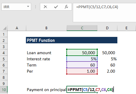
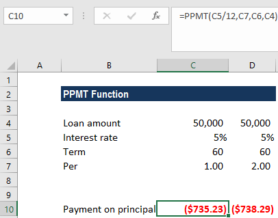
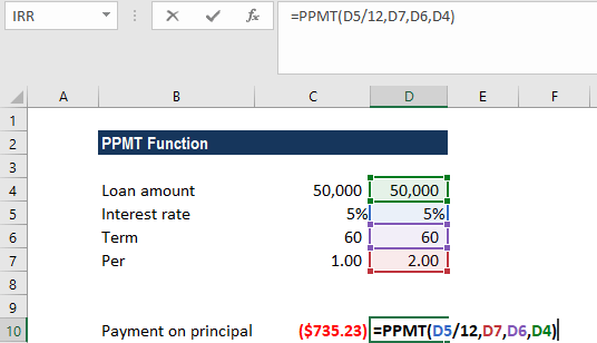
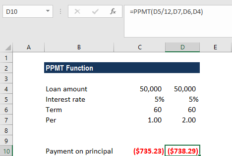
We need to calculate the payment on the principal for months 1 and 2 on a $50,000 loan, which is to be paid off in full after 5 years. Interest is charged at a rate of 5% per year and the loan repayments are to be made at the end of each month. The formula used provides a reference to the relevant cells.

We get the results below:

For month 2, we used the formula below:

We get the results below:

The above PPMT function returns the value $735.23 (rounded off to 2 decimal points). In the above example:
- We made monthly payments, so it is necessary to convert the annual interest rate of 5% into the monthly rate (=5%/12), and the number of periods from years into months (=5*12).
- Since the forecast value is zero and we need to make monthly payments, we omitted the FV and type arguments.
- We get a negative value, which signifies outgoing payments.
A few things to remember about the PPMT Function:
- #NUM! error – Occurs if the given per argument is less than 0 or is greater than the supplied value of nper.
- VALUE! error – Occurs if any of the given arguments are non-numeric.
- An error can arise if we forget to convert the interest rate or the number of periods to months or quarters when calculating monthly or quarterly payments. For the monthly rate, we need to divide the annual rate by 12, or by 4 for the quarterly rate.